In this article, we learn GCC TBC 40 wpm Statement Format.
In this blog, we will learn how to format GCC TBC English 40 wpm Statement. The formatting is as follows:
1. You have to type and format the same statement as shown on the question side of the excel sheet. You should start the statement exactly on the same cell as that of the cell on the question side of the excel sheet.
3. After that, you have to type all the column heading as shown in the question excel sheet. Type all the statements and values exactly as shown in the question side of the excel sheet and start the formatting.
4. In 40 wpm statement formatting, you have to calculate the average, sum, minimum and maximum values as asking in the question sheet by using Excel formulas.
b) Adjust the column width of the particulars properly.
c) The column width of the statistical data columns is the same, for that, you have to select those 4 columns at one time and adjust the column width equally.
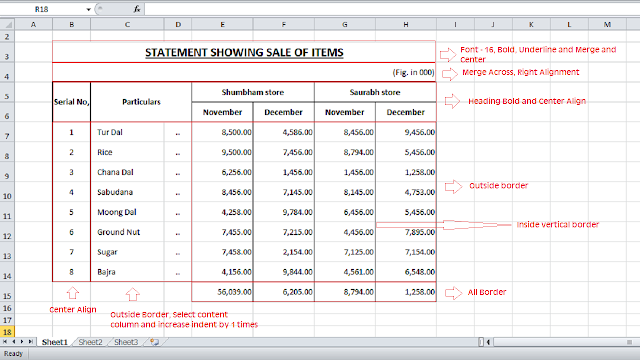
d) Select the main heading and increase its font to 16 from Home tab˃ Font Group˃ Font size and apply bold from Home tab˃ Font Group˃ Bold and underline from Home tab˃ Font Group˃ Underline and apply merge and center command from Home tab˃ Alignment group˃ Merge and center.
e) Below that row, you will get (Fig. in 000), select that row from B4 to H4 and go to Home tab˃ Alignment group˃ Merge and center and from drop-down arrow select Merge Across and apply right alignment from Home tab˃ Alignment Group˃ Right Alignment.
f) Type Particulars and all statistical data exactly the same as shown in the question side of the sheet.
g) Then select both the serial number and below this cell i.e. cell B6 and apply it Merge and center from Home tab˃ Alignment Group ˃ Merge and center and apply Bold from Home tab˃ Font Group˃ Bold. Select Particulars and below this cell i.e. cell C6 and apply Merge and center from Home tab˃ Alignment Group ˃ Merge and center and Make it Bold from Home tab˃ Font Group˃ Bold. Select two cells i.e. cell B5 and F5(Shumbhum stores) and apply Merge and center from Home tab˃ Alignment Group ˃ Merge and center and apply Bold from Home tab˃ Font Group˃ Bold and make the same formatting for Saurabh stores also i.e. cell G5 and H5.
h) Type serial number 1 in cell B7. For typing serial numbers you have to use the Fill command from Home tab˃ Editing Group˃ Fill. From the drop-down arrow of fill, you have to select series. The dialogue box of the series appears. In that dialogue box select columns in series in and give start value 1 and stop value 8 and press OK and serial numbers are automatically filled in respective column i.e. cell B8 TO B14.
i) Type the particulars as shown in the question sheet and increase its indent by pressing only one time from Home tab˃ Alignment Group˃ Increase Indent and type leader dots in column D and apply it center alignment from Home tab˃ Alignment Group˃ center alignment.
j) Main column No.1: Type the main heading in cell E5 and type its subheading in Cell E6 and E6 and apply center alignment from Home tab˃ Alignment group˃ center alignment. Select E5 and F5 both cells and apply merge and center from Home tab˃ Alignment group˃ Merge and center and Bold from Home tab˃ Font Group ˃ Bold. Type all its statistical data exactly the same as shown in the question sheet. Use a comma separator to separate the digits.
k) Main column No. 2: Type the main heading in cell G5 and type its subheading in Cell G6 and H6 and apply center alignment from Home tab˃ Alignment group˃ center alignment. Select E5 and F5 both cells and apply merge and center from Home tab˃ Alignment group˃ Merge and center and Bold from Home tab˃ Font Group ˃ Bold. Type all its statistical data exactly the same as shown in the question sheet. Use a comma separator to separate the digits.
l) Select all column heading i.e. from B5 to H6 and apply all border from the Home tab˃ Font Group ˃ Borders. Now select a cell from B7 to H14 and apply an Outside border. Select cells from C7 to D14 and apply outside border from Home tab˃ Font Group ˃ Borders. Select cells from E7 and H14 and apply inside vertical border from Home tab˃ Font Group ˃ Borders. For Inside vertical border go to Home tab˃ Font Group ˃ Borders. From the drop-down arrow of borders go to more borders, the dialogue box of format cells will be opened and from that, you have to select inside vertical border and press ok.
m) Using Excel formulas you have to calculate the values of sum, average, min, and max as asked in question in respective cells. The formula is available in Formula tab˃Function Library Group.
n) Select all statement and apply vertical middle alignment from Home tab, ˃ Alignment group, ˃vertical middle alignment and adjust row height 25 from Home tab˃ Cells group˃ Format ˃ row height.
n) Select all statement and apply vertical middle alignment from Home tab, ˃ Alignment group, ˃vertical middle alignment and adjust row height 25 from Home tab˃ Cells group˃ Format ˃ row height.
Formatted Statement of GCC TBC English 40 wpm is given below -
Marking For GCC TBC English 40 wpm statement:
The total marks for typing GCC TBC English 40 wpm statement is 5 marks. For every mistake, the half marks will be deducted, but if mistakes are 10 or more then you will get zero marks. If you start typing a statement in the wrong cell then you will also get zero marks.
Marks for Presentation:
1.Heading + Figures in Rs. – 0.5 + 0.5 Marks
2.Column heading and center alignment – 0.5 Marks
3.Other Cells Alignment – 0.5 Marks
4.Column width – 0.5 Marks
5.Borders – 0.5 Marks
6.For 4 questions on Function - 2 Marks
GCC TBC Theory-


